
Introduction
Bike-sharing demand evaluation refers back to the examine of things that impression the utilization of bike-sharing providers and the demand for bikes at totally different occasions and places. The aim of this evaluation is to grasp the patterns and traits in bike utilization and make predictions about future demand. This submit will look at how statistical machine-learning strategies can analyze the given knowledge.
This text will use a small subset of this dataset and simply give attention to the performance. Please notice that the probabilities of inaccuracy are excessive for such a small subset of the dataset. Be at liberty to make use of the whole dataset to your evaluation.
Studying Goals:
- Precisely predict the variety of bike leases for a given time interval and placement primarily based on historic knowledge and different related elements.
- Determine and analyze the important thing elements that affect bike rental demand, like climate situations, holidays, and occasions.
- Develop and consider predictive fashions that may successfully forecast bike rental demand utilizing strategies like regression evaluation, time sequence evaluation, and machine studying algorithms.
- Use the forecasting outcomes to optimize bike stock and sources, making certain that bike-sharing corporations can meet buyer demand and maximize income.
- Constantly monitor and consider the forecasting accuracy, refine the fashions, and enhance accuracy and reliability.
Dataset on Kaggle: https://www.kaggle.com/c/bike-sharing-demand
This text was printed as part of the Information Science Blogathon.
What’s Bike Sharing Demand Forecasting?
Bike-sharing demand forecasting goals to supply bike-sharing corporations with the insights and instruments they should make data-driven choices and successfully handle their operations.
Elements usually thought of throughout bike sharing demand evaluation embrace climate situations, seasonality, day of the week, vacation intervals, and occasions. Demographic details about customers, like age, gender, and revenue. It may be used to grasp utilization patterns.
Strategies utilized in bike-sharing demand evaluation embrace statistical fashions like time-series evaluation, regression evaluation, and machine studying algorithms. Bike-sharing corporations can use the evaluation outcomes to optimize their operations, distribution, pricing methods, and advertising campaigns. Moreover, the findings can inform metropolis planners in growing bike-friendly infrastructure and insurance policies.
Why Bike Sharing System?
Bike-sharing methods have turn into more and more well-liked lately as a consequence of their many advantages, which embrace:
- Inexpensive and Sustainable Transportation: Bike-sharing methods present an inexpensive and sustainable mode of transportation, particularly for brief journeys. They’re a low-cost various to proudly owning a private bike and may help scale back reliance on non-public vehicles and sharing vehicles, which might positively impression the setting.
- Well being and luxury: Bike-sharing methods promote bodily motion and train, positively impacting well being and luxury. Common biking may help scale back the danger of coronary heart illness, stroke, and different persistent ailments.
- Comfort: Bike-sharing methods are sometimes situated in densely populated metropolis areas, making them a handy mode of transportation for brief journeys. They are often simply accessed, making them a versatile and handy choice for commuters and vacationers alike.
- Decreased Site visitors Congestion: Bike-sharing methods may help scale back visitors congestion by offering an alternate mode of transportation for brief journeys. This will have a optimistic impression on city mobility.
In abstract, bike-sharing methods present a number of advantages, together with inexpensive and sustainable transportation, well being and luxury, comfort, lowered visitors congestion, and tourism and financial growth. These advantages have contributed to the recognition of bike-sharing methods in lots of cities all over the world.
Downside Assertion
The issue assertion for bike-sharing demand is predicting the variety of bikes that will likely be rented from a bike-sharing system at a given time primarily based on elements reminiscent of climate, day of the week, and time of day. The aim is to construct a predictive mannequin that may precisely forecast bike rental demand to optimize bike allocation and enhance the bike-sharing system’s general effectivity.
The issue assertion could contain answering particular questions reminiscent of:
- What’s the anticipated demand for bikes throughout peak hours, weekdays, or weekends?
- How does climate (e.g., wind, temperature, precipitation) have an effect on bike rental demand?
- Are any particular places or routes with larger or decrease demand for bikes?
- How can we optimize the bike-sharing system to fulfill fluctuating demand and decrease operational prices?
- Can the bike-sharing system increase or enhance to higher serve customers’ wants and promote sustainable transportation?
The issue assertion for bike-sharing demand evaluation sometimes includes predicting bike rental demand and optimizing bike allocation to enhance the bike-sharing system’s effectivity and sustainability.
The corporate administration needs:
- To create a mannequin of the demand for shared bikes with the obtainable unbiased variables.
- To grasp the demand dynamics of the market utilizing the mannequin.
Studying and Understanding the Information
To construct a bike-sharing demand forecasting mannequin, it’s vital to start out by studying and understanding the information. The important thing steps concerned on this course of are loading, exploring, cleansing, preprocessing, and visualizing the information. By following these steps, analysts can acquire a deeper understanding of the information and establish any points that want addressing earlier than constructing the bike-sharing demand forecasting mannequin. This helps make sure the mannequin is correct and dependable, which is important for optimizing bike-sharing operations.
import pandas as pd

bikeshare_df = pd.read_csv("day.csv")

print(bikeshare_df.head())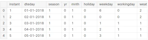
bike_sharing.data()
bike_sharing.describe()

Visualizing the Information
Visualizing the information is a vital step within the bike-sharing demand forecasting course of. It could actually assist establish patterns and traits that is probably not instantly obvious from uncooked knowledge.
import matplotlib.pyplot as plt
import seaborn as sns


#Plotting pairplot of all of the numeric variables

sns.pairplot(bike_sharing[["temp","atemp","hum","windspeed","casual","registered","cnt"]])
plt.present()

#Plotting field plot of steady variables

plt.determine(figsize=(20, 12))
plt.subplot(2,3,1)
plt.boxplot(bike_sharing["temp"])
plt.subplot(2,3,2)
plt.boxplot(bike_sharing["atemp"])
plt.subplot(2,3,3)
plt.boxplot(bike_sharing["hum"])
plt.subplot(2,3,4)
plt.boxplot(bike_sharing["windspeed"])
plt.subplot(2,3,5)
plt.boxplot(bike_sharing["casual"])
plt.subplot(2,3,6)
plt.boxplot(bike_sharing["registered"])
plt.present()
Visualising Categorical Variables
#Plotting field plot of categorical variables

plt.determine(figsize=(20, 12))
plt.subplot(3,3,1)
sns.boxplot(x = 'season', y = 'cnt', knowledge = bike_sharing)
plt.subplot(3,3,2)
sns.boxplot(x = 'yr', y = 'cnt', knowledge = bike_sharing)
plt.subplot(3,3,3)
sns.boxplot(x = 'mnth', y = 'cnt', knowledge = bike_sharing)
plt.subplot(3,3,4)
sns.boxplot(x = 'vacation', y = 'cnt', knowledge = bike_sharing)
plt.subplot(3,3,5)
sns.boxplot(x = 'weekday', y = 'cnt', knowledge = bike_sharing)
plt.subplot(3,3,6)
sns.boxplot(x = 'workingday', y = 'cnt', knowledge = bike_sharing)
plt.subplot(3,3,7)
sns.boxplot(x = 'weathersit', y = 'cnt', knowledge = bike_sharing)
plt.present()
Information Preparation
Information preparation is an important step in bike-sharing demand forecasting, because it includes cleansing, remodeling, and organizing the information to make it appropriate for evaluation. By making ready the information on this method, analysts can make sure that the information is appropriate for evaluation and that any biases or errors within the knowledge are addressed. This will result in extra correct and dependable forecasting fashions that may assist bike-sharing corporations optimize their operations and higher meet buyer demand.
Dropping pointless columns immediate, dteday, informal & registered
- immediate – It’s only a sequence variety of rows
- dteday – It’s not required since columns for 12 months & month already exists
- informal – This variable can’t be predicted.
- registered – This variable can’t be predicted.
bike_sharing.drop(columns=["instant","dteday","casual","registered"],axis=1,inplace =True)
bike_sharing.head()
Dummy Variables
season_type = pd.get_dummies(bike_sharing['season'], drop_first = True)
season_type.rename(columns={2:"season_summer", 3:"season_fall", 4:"season_winter"},inplace=True)
season_type.head()

weather_type = pd.get_dummies(bike_sharing['weathersit'], drop_first = True)
weather_type.rename(columns={2:"weather_mist_cloud", 3:"weather_light_snow_rain"},inplace=True)
weather_type.head()

#Concatenating new dummy variables to the primary dataframe

bike_sharing = pd.concat([bike_sharing, season_type, weather_type], axis = 1)

#Dropping columns season & weathersit since we have now already created dummies for them

bike_sharing.drop(columns=["season", "weathersit"],axis=1,inplace =True)

#Analysing dataframe after dropping columns

bike_sharing.data()

Creating derived variables for the explicit variable month
#Creating year_quarter derived columns from month columns.
#Word that final quarter has not been created since we want solely 3 columns to outline the 4 quarters.

bike_sharing["Quarter_JanFebMar"] = bike_sharing["mnth"].apply(lambda x: 1 if x<=3 else 0)
bike_sharing["Quarter_AprMayJun"] = bike_sharing["mnth"].apply(lambda x: 1 if 4<=x<=6 else 0)
bike_sharing["Quarter_JulAugSep"] = bike_sharing["mnth"].apply(lambda x: 1 if 7<=x<=9 else 0)

#Dropping column mnth since we have now already created dummies.

bike_sharing.drop(columns=["mnth"],axis=1,inplace =True)
bike_sharing["weekend"] = bike_sharing["weekday"].apply(lambda x: 0 if 1<=x<=5 else 1)
bike_sharing.drop(columns=["weekday"],axis=1,inplace =True)
bike_sharing.drop(columns=["workingday"],axis=1,inplace =True)
bike_sharing.head()

#Analysing dataframe after dropping columns weekday & workingday

bike_sharing.data()
#Plotting correlation heatmap to investigate the linearity between the variables within the dataframe

plt.determine(figsize = (16, 10))
sns.heatmap(bike_sharing.corr(), annot = True, cmap="Greens")
plt.present()
#Dropping column temp since it is extremely extremely collinear with the column atemp.
#Additional,the column atemp is extra applicable for modelling in comparison with column temp from human perspective.

bike_sharing.drop(columns=["temp"],axis=1,inplace =True)
bike_sharing.head()
Splitting the Information into Coaching and Testing Units
Splitting the information into coaching and testing units is a essential step in bike-sharing demand forecasting. It allows analysts to judge the efficiency of their forecasting fashions on unseen knowledge. The overall strategy is to make use of historic knowledge to coach the mannequin after which check the mannequin’s efficiency on a separate, holdout set of knowledge.
#Importing library

from sklearn.model_selection import train_test_split

# We specify this in order that the practice and check knowledge set all the time have the identical rows, respectively
np.random.seed(0)
bike_sharing_train, bike_sharing_test = train_test_split(bike_sharing, train_size = 0.7, test_size = 0.3, random_state = 100)
Rescaling the coaching dataframe utilizing the MinMax scaling perform after the cut up to realize optimum beta coefficients for all options.
#importing library
from sklearn.preprocessing import MinMaxScaler

#assigning variable to scaler
scaler = MinMaxScaler()
# Making use of scaler to all of the columns besides the derived and 'dummy' variables which can be already in 0 & 1.

numeric_var = ['atemp','hum','windspeed','cnt']
bike_sharing_train[numeric_var] = scaler.fit_transform(bike_sharing_train[numeric_var])

# Analysing the practice dataframe after scaling
bike_sharing_train.head()
By splitting the information into coaching and testing units, analysts can consider the efficiency of their forecasting fashions on unseen knowledge and make sure that the fashions are sturdy and dependable. This may help bike-sharing corporations optimize their operations and higher meet buyer demand.
y_train = bike_sharing_train.pop('cnt')
X_train = bike_sharing_train

print (y_train.head())
print (X_train.head())
Constructing the Linear Mannequin
Constructing a linear mannequin for bike-sharing demand forecasting includes making a mannequin that makes use of linear regression to foretell bike rental demand primarily based on a set of enter variables. The linear regression mannequin is skilled utilizing the coaching set, with the enter variables used to foretell the goal variable (bike rental demand). The mannequin is optimized to reduce the error between the expected and precise calls for within the coaching set.
Utilizing the LinearRegression perform from SciKit Study and Recursive Function Elimination (RFE):
# Importing RFE and LinearRegression
from sklearn.feature_selection import RFE
from sklearn.linear_model import LinearRegression
# Working RFE with the output variety of the variable equal to 12
lm = LinearRegression()
lm.match(X_train, y_train)

rfe = RFE(lm, 12)             # working RFE
rfe = rfe.match(X_train, y_train)

listing(zip(X_train.columns,rfe.support_,rfe.ranking_))

By constructing a linear mannequin for bike-sharing demand forecasting, analysts can develop a easy but efficient forecasting system to optimize bike-sharing operations and enhance buyer satisfaction. Nonetheless, it’s vital to notice that linear fashions could have limitations in capturing extra complicated patterns and relationships within the knowledge, so different modeling strategies (reminiscent of choice bushes or neural networks) might be extra correct predictions.
# Creating X_test dataframe with RFE chosen variables
X_train_rfe = X_train[columns_rfe]
X_train_rfe
Residual Evaluation of the Coaching Information
Residual evaluation is a necessary step in evaluating the efficiency of a linear mannequin for bike-sharing demand forecasting. Residuals are the distinction between the expected demand and the precise demand, and analyzing these residuals may help establish any patterns or biases within the mannequin’s predictions.
#utilizing the ultimate mannequin lr5 on practice knowledge to foretell y_train_cnt values
y_train_cnt = lr5.predict(X_train_lr5)
# Plotting the histogram of the error phrases
fig = plt.determine()
sns.distplot((y_train - y_train_cnt), bins = 20)
fig.suptitle('Error Phrases', fontsize = 20)
plt.xlabel('Errors', fontsize = 18)
plt.scatter(y_train,(y_train - y_train_cnt))
plt.present()
Making Predictions Utilizing the Closing Mannequin lr5
To make predictions utilizing the ultimate linear mannequin for bike-sharing demand forecasting (lr5), you will want to supply values for the enter variables and use the mannequin to generate a prediction for the goal variable (bike rental demand).
#Making use of the scaling on the check units

numeric_vars = ['atemp','hum','windspeed','cnt']
bike_sharing_test[numeric_vars] = scaler.remodel(bike_sharing_test[numeric_vars])

bike_sharing_test.describe()

Dividing into X_test and y_test
y_test = bike_sharing_test.pop('cnt')
X_test = bike_sharing_test

# Including fixed variable to check dataframe
X_test_lr5 = sm.add_constant(X_test)

# Updating X_test_lr5 dataframe by dropping the variables as analyzed from the above fashions

X_test_lr5 =X_test_lr5.drop(["atemp", "hum", "season_fall", "Quarter_AprMayJun", "weekend","Quarter_JanFebMar"], axis = 1)

# Making predictions utilizing the fifth mannequin

y_pred = lr5.predict(X_test_lr5)
Mannequin Analysis
Mannequin analysis is a essential step in assessing the efficiency of a bike-sharing demand forecasting mannequin. Use numerous metrics to judge the efficiency of a mannequin, together with imply absolute error (MAE), root imply squared error (RMSE), and coefficient of dedication (R-squared).
# Plotting y_test and y_pred to grasp the unfold

fig = plt.determine()
plt.scatter(y_test, y_pred)
fig.suptitle('y_test vs y_pred', fontsize = 20)
plt.xlabel('y_test', fontsize = 18)

plt.ylabel('y_pred', fontsize = 16)

It’s best to consider the mannequin’s efficiency utilizing metrics reminiscent of MAE, RMSE, and R-squared. MAE and RMSE measure the common magnitude of the errors between the expected and precise values. R-squared measures the proportion of variance within the goal variable, defined by the enter variables.
#importing library and checking imply squared error
from sklearn.metrics import mean_squared_error

mse = mean_squared_error(y_test, y_pred)
print('Mean_Squared_Error :' ,mse)

#importing library and checking R2

from sklearn.metrics import r2_score
r2_score(y_test, y_pred)

Conclusion
This examine aimed to enhance the bike-sharing actions of Capital Bikeshare and assist the reinvention of the town transportation system. This complete exploratory knowledge evaluation on their publicly obtainable knowledge helped us perceive and analyze the underlying patterns and traits of the bike-share community and to work on this knowledge to realize data-driven outcomes.
We carried out an evaluation on the expansion in recognition of bike-share over the 2 years, 2011–2012, and the impact of the seasonal and day elements on the ridership patterns. The impacts of seasonal and climate parameters have been to grasp the ridership sample in Washington, DC. Evaluation of the journey knowledge helped to grasp the traits of the locality the place the stations are situated.
Protecting these inferences in thoughts, we may counsel the next suggestions:
- Many of the leases are for commuting to workshops and schools each day. So CaBi ought to launch extra stations close to these landmarks to achieve out to their foremost prospects.
- Planning for extra sharing bikes to stations should contemplate the height rental hours, i.e., 7–9 am and 5–6 pm.
- The provide shouldn’t be a set worth. As an alternative, it ought to be primarily based on differences due to the season to advertise bike utilization in the course of the fall and winter seasons.
- Information about essentially the most used routes may help construct roads/lanes devoted to bikes particularly.
- Because of the low utilization of bikes at evening, it might be higher to do bike upkeep at evening. Eradicating some bikes from the streets at evening time won’t trigger hassle for the purchasers.
- Changing registered prospects to informal prospects on the weekends by offering them with reductions and coupons.
The media proven on this article just isn’t owned by Analytics Vidhya and is used on the Creator’s discretion.